Visualizing Data For Regression
read.auto <- function(file = 'Automobile price data _Raw_.csv'){
    ## Read the csv file
    auto.price <- read.csv(file, header = TRUE, stringsAsFactors = FALSE)

    numcols <- switch(
      as.character((!exists("numcols") || is.na(numcols) || is.null(numcols))[1]),
      "TRUE" = { # if numcols does not exist or is not populated ("TRUE"),
        # use these defaults:
        c('price', 'bore', 'stroke', 'horsepower', 'peak.rpm')
      }, # else use existing values
      numcols)
    print(c("numeric columns:", numcols))

    for(col in c('price', 'bore', 'stroke', 'horsepower', 'peak.rpm')){
        for (idx in (1:length(auto.price[,col]))) {
          temp = auto.price[idx,col]
          if (temp == '?' || is.na(auto.price[idx,col])) {
            # Convert ? to NA
            auto.price[idx,col] = ifelse(temp == '?', NA, auto.price[idx,col])
            print(c(col, idx, auto.price[idx,col]))
          }
        }

        ## Coerce some character columns to numeric
        auto.price[,col] = as.numeric(auto.price[,col])
    }

    ## Remove cases or rows with missing values.
    ## Keep the rows which do not have NAs.
    auto.price = auto.price[complete.cases(auto.price[, numcols]), ]

    ## Drop some unneeded columns
    auto.price[,'symboling'] = NULL
    auto.price[,'normalized.losses'] = NULL

    return(auto.price)
}

cat_cols <- c('fuel.type', 'aspiration', 'num.of.doors', 'body.style',
            'drive.wheels', 'engine.location', 'engine.type', 'num.of.cylinders')

plotcols <- c('price', 'city.mpg', 'curb.weight', 'engine.size', 'horsepower', 'fuel.type')

auto_prices <- read.auto()
## [1] "numeric columns:" "price"            "bore"             "stroke"
## [5] "horsepower"       "peak.rpm"
## [1] "price" "10"    NA
## [1] "price" "45"    NA
## [1] "price" "46"    NA
## [1] "price" "130"   NA
## [1] "bore" "56"   NA
## [1] "bore" "57"   NA
## [1] "bore" "58"   NA
## [1] "bore" "59"   NA
## [1] "stroke" "56"     NA
## [1] "stroke" "57"     NA
## [1] "stroke" "58"     NA
## [1] "stroke" "59"     NA
## [1] "horsepower" "131"        NA
## [1] "horsepower" "132"        NA
## [1] "peak.rpm" "131"      NA
## [1] "peak.rpm" "132"      NA
print("all auto columns:")
## [1] "all auto columns:"
colnames(auto_prices)
##  [1] "make"              "fuel.type"         "aspiration"
##  [4] "num.of.doors"      "body.style"        "drive.wheels"
##  [7] "engine.location"   "wheel.base"        "length"
## [10] "width"             "height"            "curb.weight"
## [13] "engine.type"       "num.of.cylinders"  "engine.size"
## [16] "fuel.system"       "bore"              "stroke"
## [19] "compression.ratio" "horsepower"        "peak.rpm"
## [22] "city.mpg"          "highway.mpg"       "price"
head(auto_prices)
##          make fuel.type aspiration num.of.doors  body.style drive.wheels
## 1 alfa-romero       gas        std          two convertible          rwd
## 2 alfa-romero       gas        std          two convertible          rwd
## 3 alfa-romero       gas        std          two   hatchback          rwd
## 4        audi       gas        std         four       sedan          fwd
## 5        audi       gas        std         four       sedan          4wd
## 6        audi       gas        std          two       sedan          fwd
##   engine.location wheel.base length width height curb.weight engine.type
## 1           front       88.6  168.8  64.1   48.8        2548        dohc
## 2           front       88.6  168.8  64.1   48.8        2548        dohc
## 3           front       94.5  171.2  65.5   52.4        2823        ohcv
## 4           front       99.8  176.6  66.2   54.3        2337         ohc
## 5           front       99.4  176.6  66.4   54.3        2824         ohc
## 6           front       99.8  177.3  66.3   53.1        2507         ohc
##   num.of.cylinders engine.size fuel.system bore stroke compression.ratio
## 1             four         130        mpfi 3.47   2.68               9.0
## 2             four         130        mpfi 3.47   2.68               9.0
## 3              six         152        mpfi 2.68   3.47               9.0
## 4             four         109        mpfi 3.19   3.40              10.0
## 5             five         136        mpfi 3.19   3.40               8.0
## 6             five         136        mpfi 3.19   3.40               8.5
##   horsepower peak.rpm city.mpg highway.mpg price
## 1        111     5000       21          27 13495
## 2        111     5000       21          27 16500
## 3        154     5000       19          26 16500
## 4        102     5500       24          30 13950
## 5        115     5500       18          22 17450
## 6        110     5500       19          25 15250
str(auto_prices)
## 'data.frame':    195 obs. of  24 variables:
##  $ make             : chr  "alfa-romero" "alfa-romero" "alfa-romero" "audi" ...
##  $ fuel.type        : chr  "gas" "gas" "gas" "gas" ...
##  $ aspiration       : chr  "std" "std" "std" "std" ...
##  $ num.of.doors     : chr  "two" "two" "two" "four" ...
##  $ body.style       : chr  "convertible" "convertible" "hatchback" "sedan" ...
##  $ drive.wheels     : chr  "rwd" "rwd" "rwd" "fwd" ...
##  $ engine.location  : chr  "front" "front" "front" "front" ...
##  $ wheel.base       : num  88.6 88.6 94.5 99.8 99.4 ...
##  $ length           : num  169 169 171 177 177 ...
##  $ width            : num  64.1 64.1 65.5 66.2 66.4 66.3 71.4 71.4 71.4 64.8 ...
##  $ height           : num  48.8 48.8 52.4 54.3 54.3 53.1 55.7 55.7 55.9 54.3 ...
##  $ curb.weight      : int  2548 2548 2823 2337 2824 2507 2844 2954 3086 2395 ...
##  $ engine.type      : chr  "dohc" "dohc" "ohcv" "ohc" ...
##  $ num.of.cylinders : chr  "four" "four" "six" "four" ...
##  $ engine.size      : int  130 130 152 109 136 136 136 136 131 108 ...
##  $ fuel.system      : chr  "mpfi" "mpfi" "mpfi" "mpfi" ...
##  $ bore             : num  3.47 3.47 2.68 3.19 3.19 3.19 3.19 3.19 3.13 3.5 ...
##  $ stroke           : num  2.68 2.68 3.47 3.4 3.4 3.4 3.4 3.4 3.4 2.8 ...
##  $ compression.ratio: num  9 9 9 10 8 8.5 8.5 8.5 8.3 8.8 ...
##  $ horsepower       : num  111 111 154 102 115 110 110 110 140 101 ...
##  $ peak.rpm         : num  5000 5000 5000 5500 5500 5500 5500 5500 5500 5800 ...
##  $ city.mpg         : int  21 21 19 24 18 19 19 19 17 23 ...
##  $ highway.mpg      : int  27 27 26 30 22 25 25 25 20 29 ...
##  $ price            : num  13495 16500 16500 13950 17450 ...
summary(auto_prices)
##      make            fuel.type          aspiration        num.of.doors
##  Length:195         Length:195         Length:195         Length:195
##  Class :character   Class :character   Class :character   Class :character
##  Mode  :character   Mode  :character   Mode  :character   Mode  :character
##
##
##
##   body.style        drive.wheels       engine.location      wheel.base
##  Length:195         Length:195         Length:195         Min.   : 86.6
##  Class :character   Class :character   Class :character   1st Qu.: 94.5
##  Mode  :character   Mode  :character   Mode  :character   Median : 97.0
##                                                           Mean   : 98.9
##                                                           3rd Qu.:102.4
##                                                           Max.   :120.9
##      length          width           height       curb.weight
##  Min.   :141.1   Min.   :60.30   Min.   :47.80   Min.   :1488
##  1st Qu.:166.3   1st Qu.:64.05   1st Qu.:52.00   1st Qu.:2145
##  Median :173.2   Median :65.40   Median :54.10   Median :2414
##  Mean   :174.3   Mean   :65.89   Mean   :53.86   Mean   :2559
##  3rd Qu.:184.1   3rd Qu.:66.90   3rd Qu.:55.65   3rd Qu.:2944
##  Max.   :208.1   Max.   :72.00   Max.   :59.80   Max.   :4066
##  engine.type        num.of.cylinders    engine.size    fuel.system
##  Length:195         Length:195         Min.   : 61.0   Length:195
##  Class :character   Class :character   1st Qu.: 98.0   Class :character
##  Mode  :character   Mode  :character   Median :120.0   Mode  :character
##                                        Mean   :127.9
##                                        3rd Qu.:145.5
##                                        Max.   :326.0
##       bore           stroke     compression.ratio   horsepower
##  Min.   :2.540   Min.   :2.07   Min.   : 7.00     Min.   : 48.0
##  1st Qu.:3.150   1st Qu.:3.11   1st Qu.: 8.50     1st Qu.: 70.0
##  Median :3.310   Median :3.29   Median : 9.00     Median : 95.0
##  Mean   :3.329   Mean   :3.25   Mean   :10.19     Mean   :103.3
##  3rd Qu.:3.590   3rd Qu.:3.41   3rd Qu.: 9.40     3rd Qu.:116.0
##  Max.   :3.940   Max.   :4.17   Max.   :23.00     Max.   :262.0
##     peak.rpm       city.mpg      highway.mpg        price
##  Min.   :4150   Min.   :13.00   Min.   :16.00   Min.   : 5118
##  1st Qu.:4800   1st Qu.:19.50   1st Qu.:25.00   1st Qu.: 7756
##  Median :5100   Median :25.00   Median :30.00   Median :10245
##  Mean   :5099   Mean   :25.37   Mean   :30.84   Mean   :13248
##  3rd Qu.:5500   3rd Qu.:30.00   3rd Qu.:35.00   3rd Qu.:16509
##  Max.   :6600   Max.   :49.00   Max.   :54.00   Max.   :45400
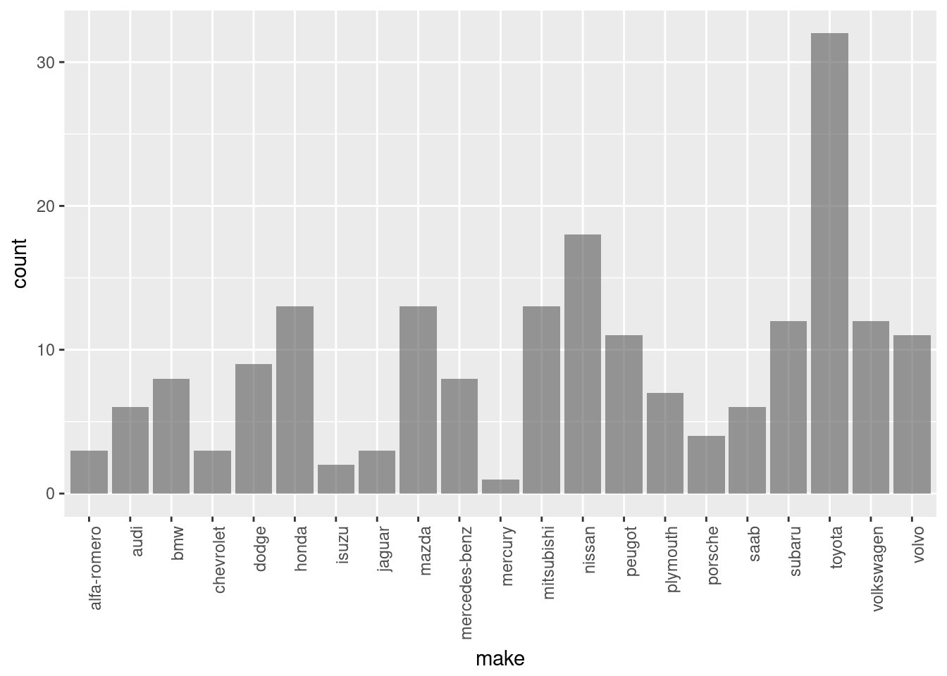
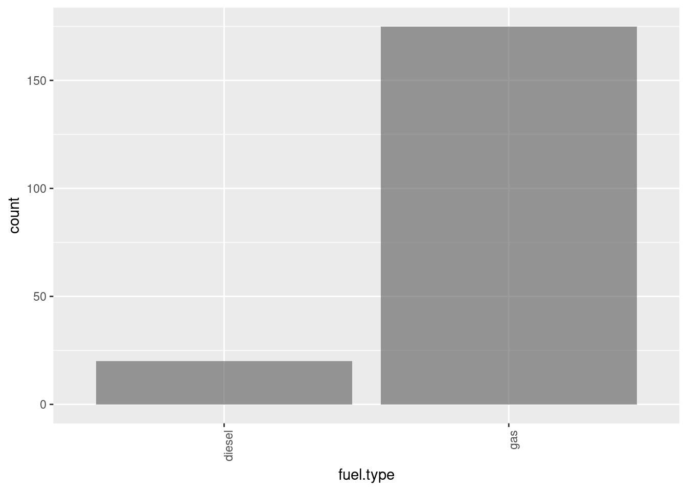
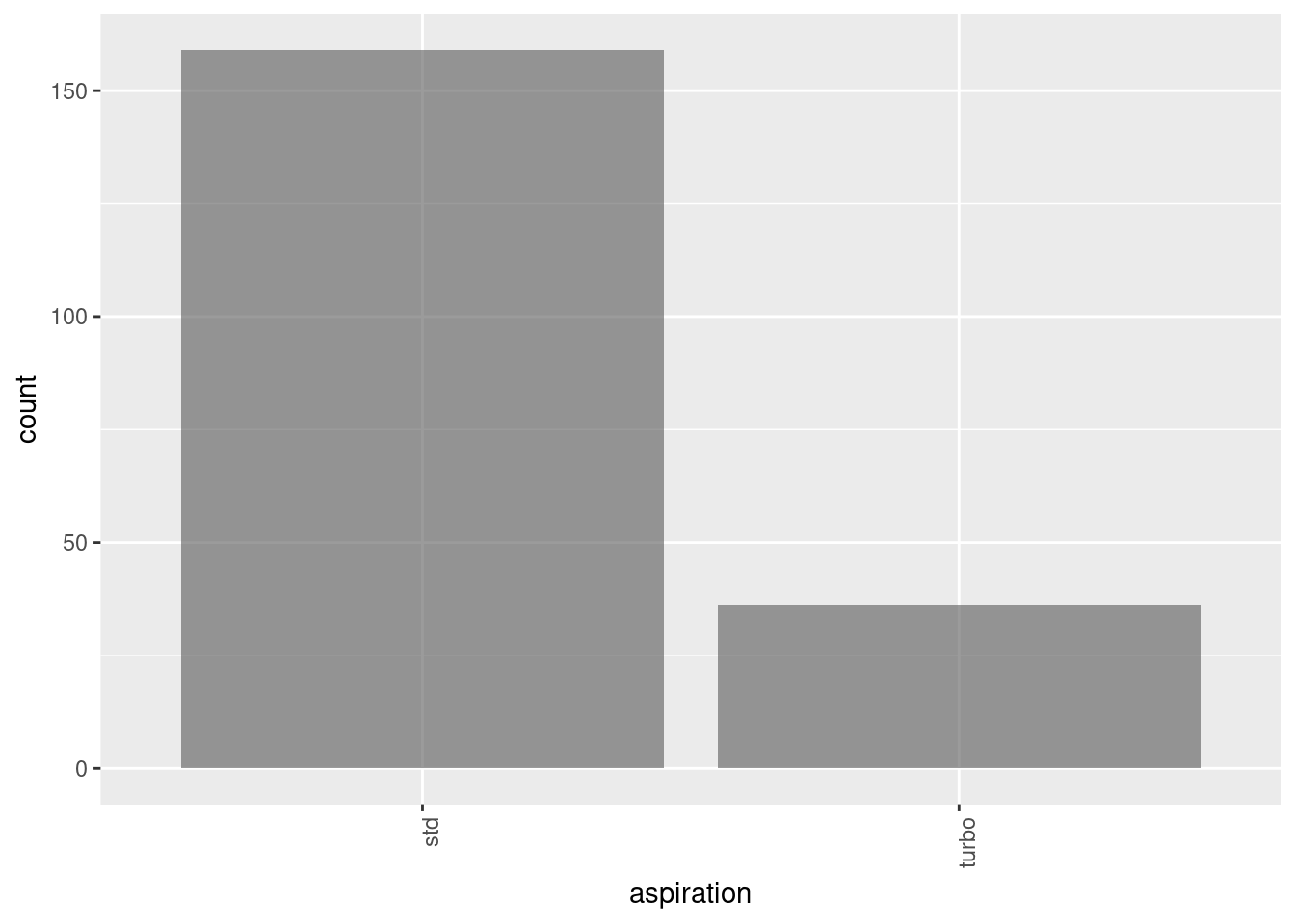
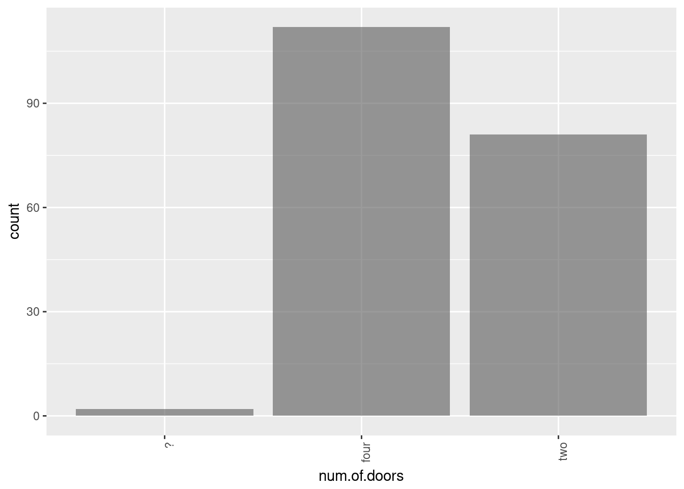
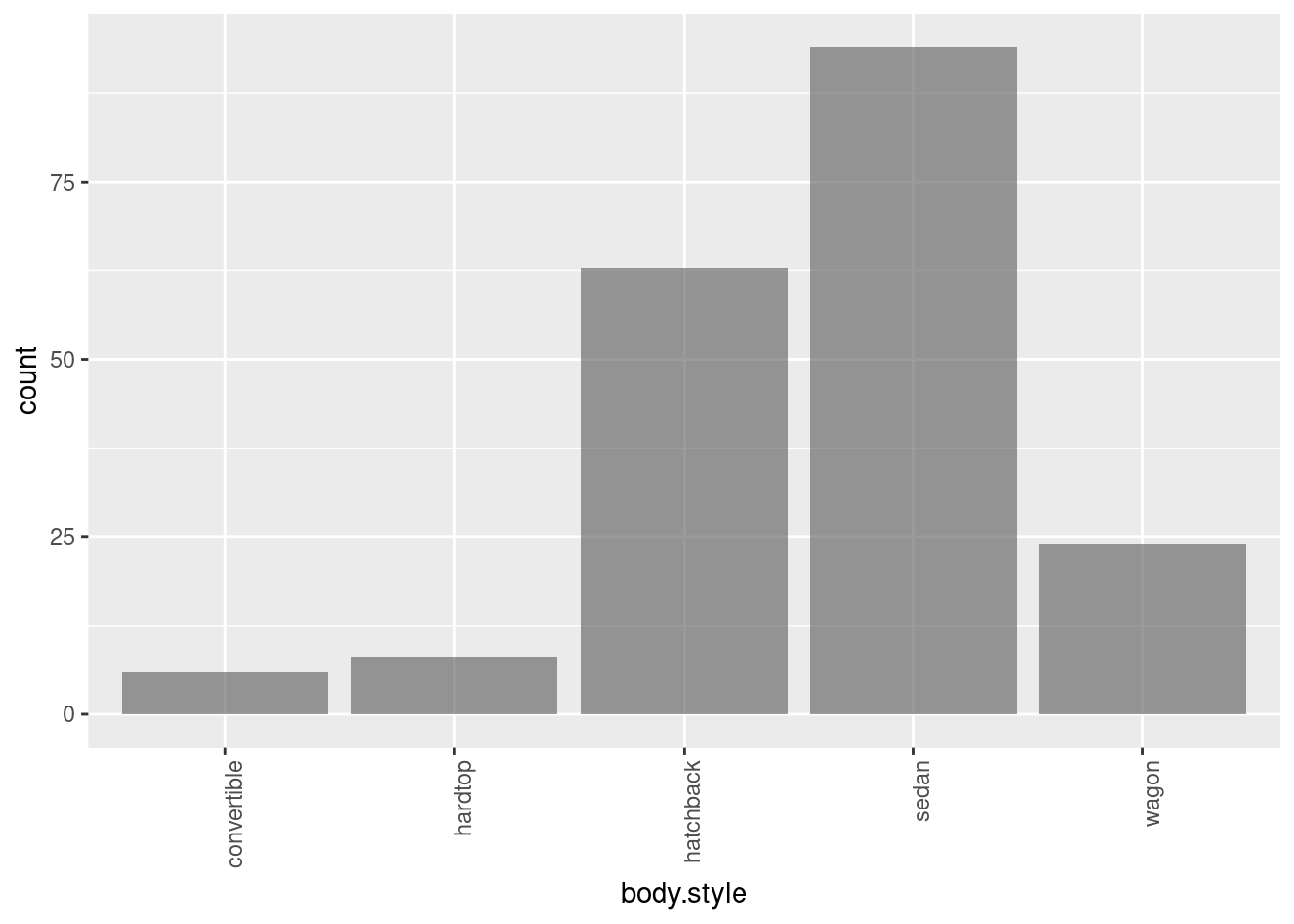
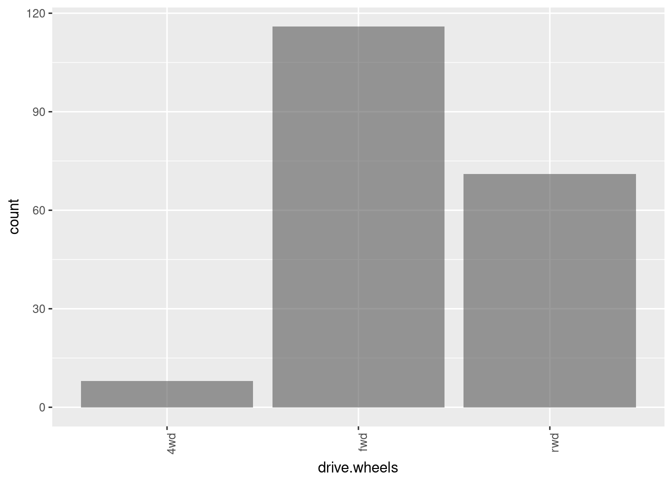
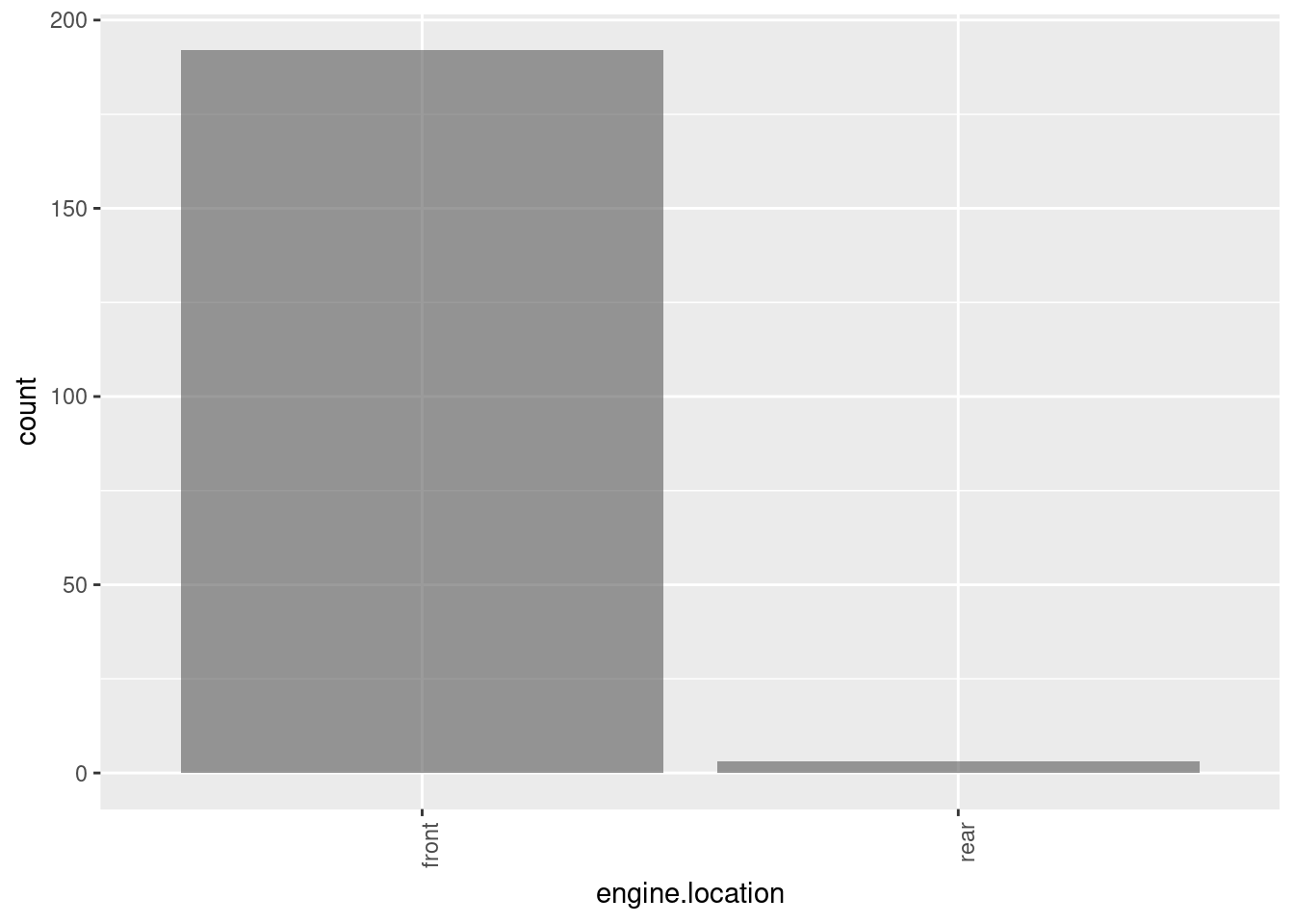
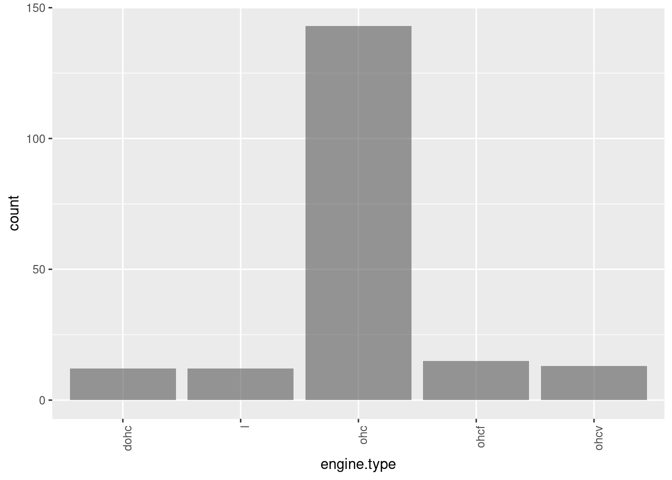
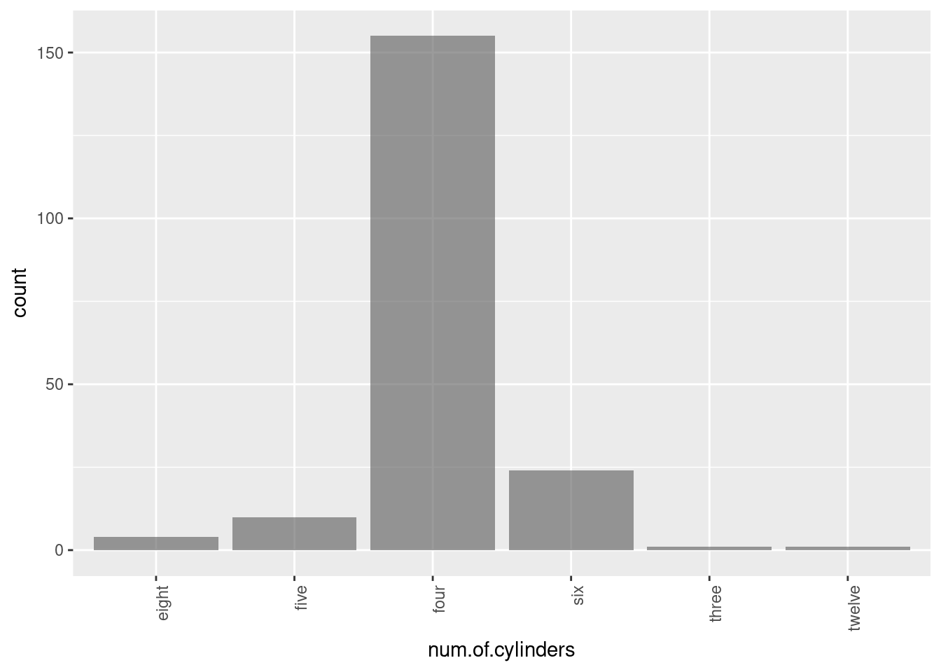
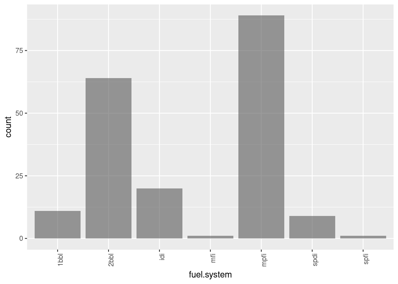
plot_bars <- function(df){
    options(repr.plot.width=4, repr.plot.height=3.5) # Set the initial plot area dimensions

    print("character columns:")
    for(col in colnames(df)){
        if(is.character(df[,col])){
            print(col)
            p <- ggplot(df, aes_string(col)) +
                       geom_bar(alpha = 0.6) +
                       theme(axis.text.x = element_text(angle = 90, hjust = 1))
            print(p)
        }
    }
}

plot_bars(auto_prices)
## [1] "character columns:"
## [1] "make"
## [1] "fuel.type"
## [1] "aspiration"
## [1] "num.of.doors"
## [1] "body.style"
## [1] "drive.wheels"
## [1] "engine.location"
## [1] "engine.type"
## [1] "num.of.cylinders"
## [1] "fuel.system"
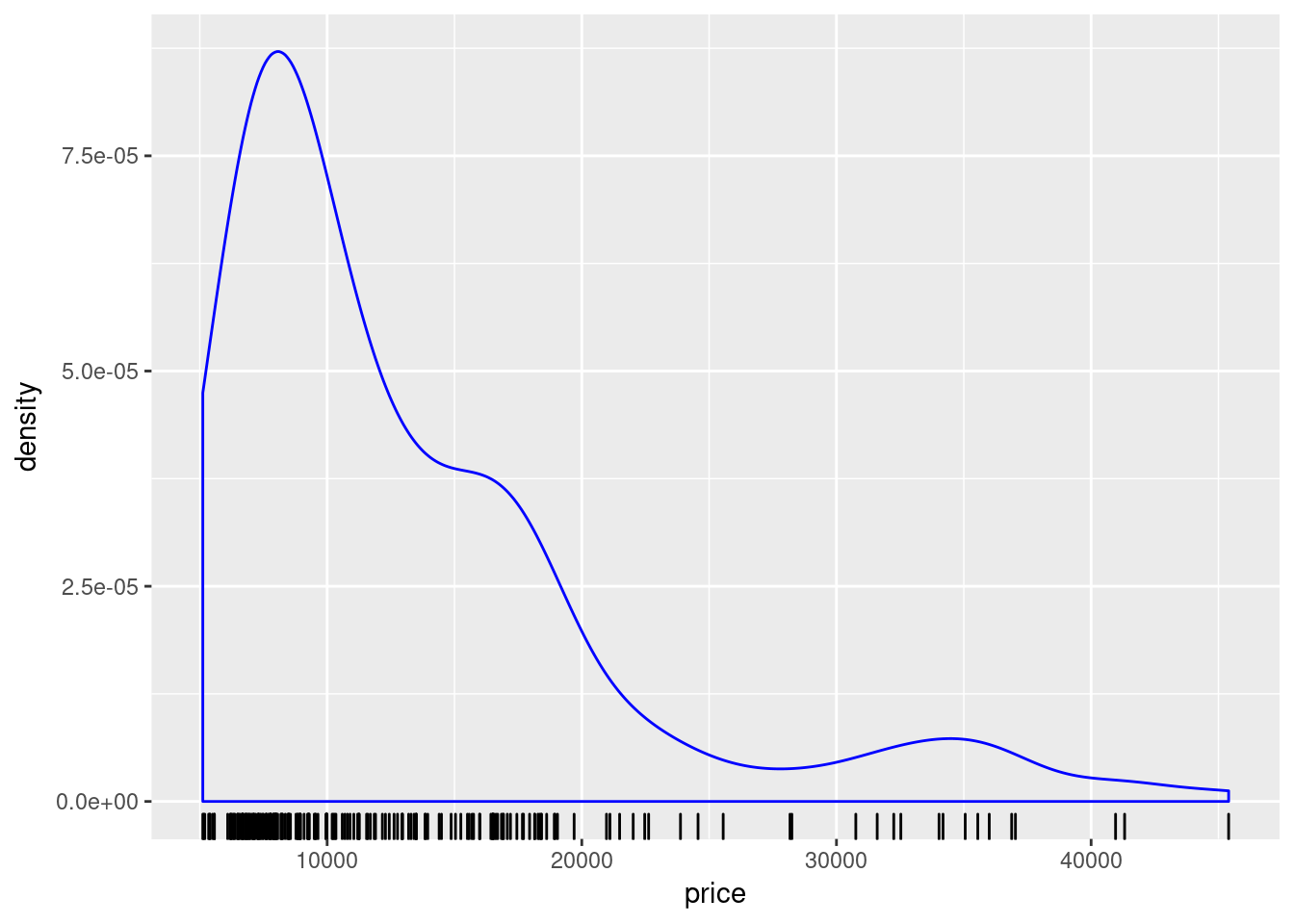
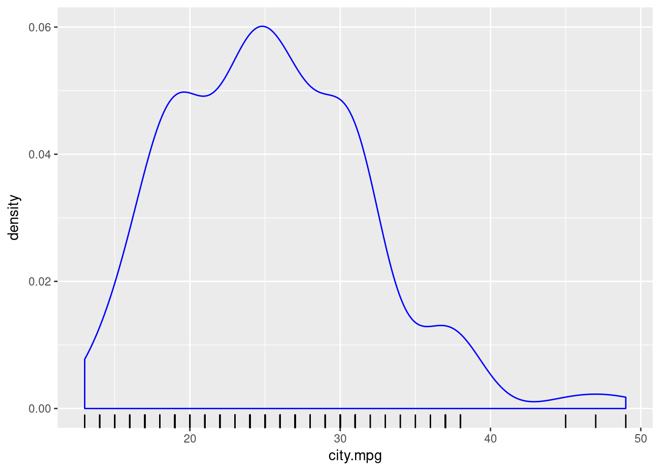
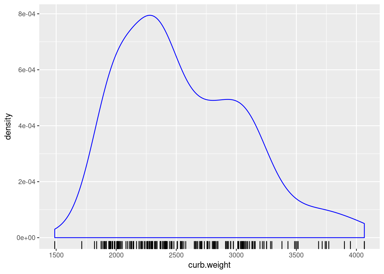
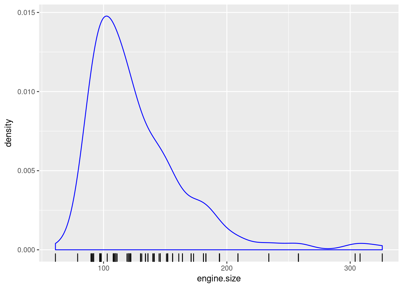
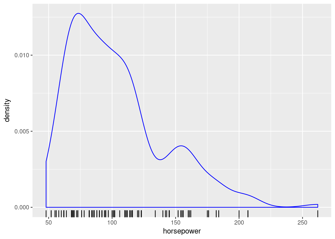
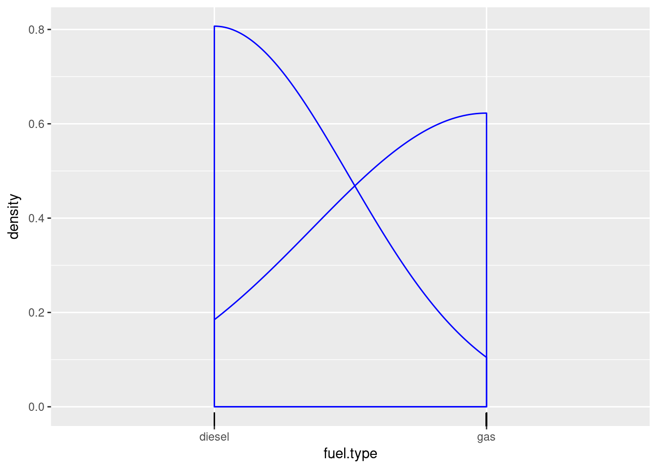
plot_dist <- function(df, plotcols){
    options(repr.plot.width=4, repr.plot.height=3) # Set the initial plot area dimensions
    for(col in plotcols){
        #if(is.numeric(df[,col])){
            p <- ggplot(df, aes_string(col)) +
                       geom_density(color = 'blue') +
                       geom_rug()
            print(p)
        #}
    }
}

plot_dist(auto_prices, plotcols)
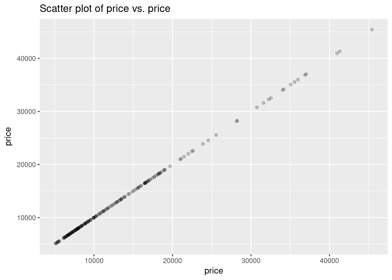
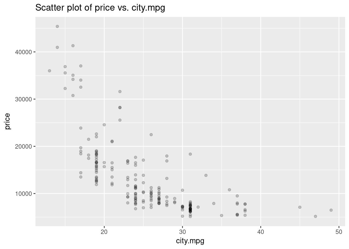
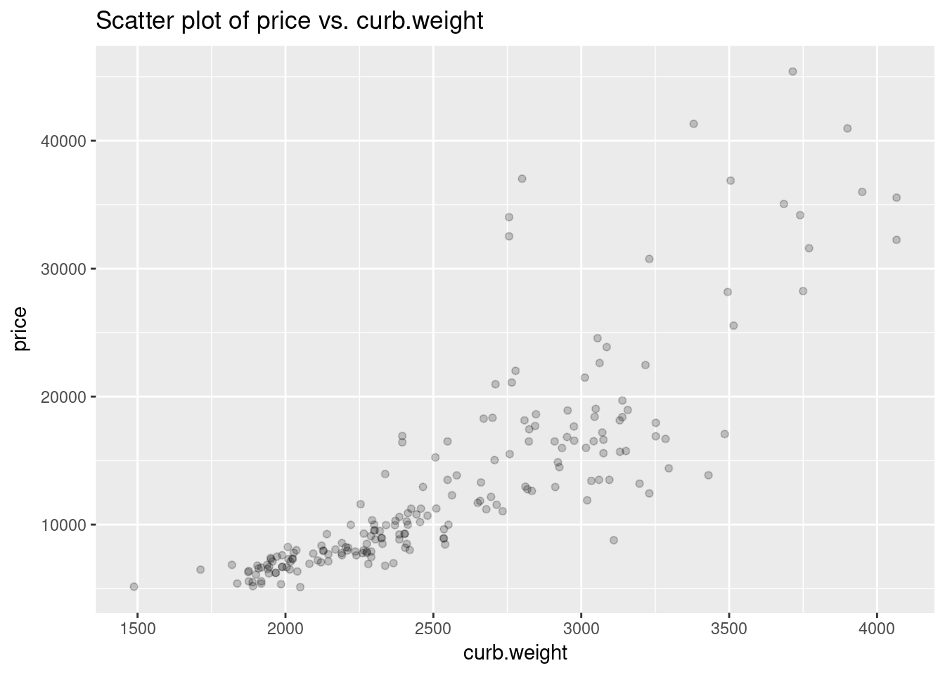
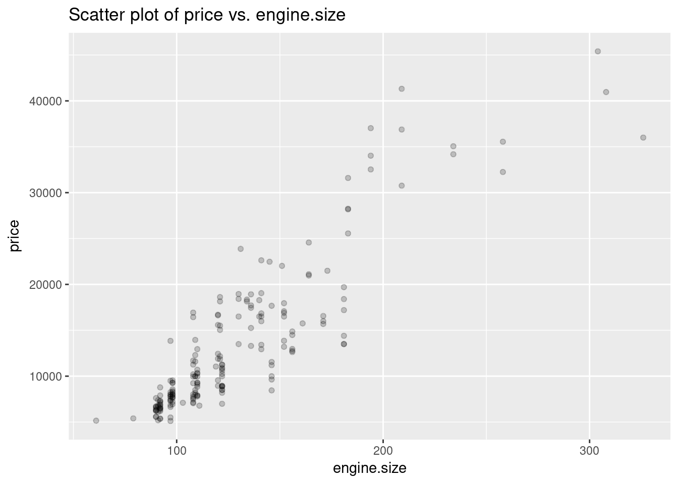
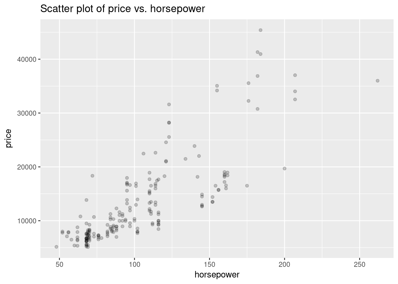
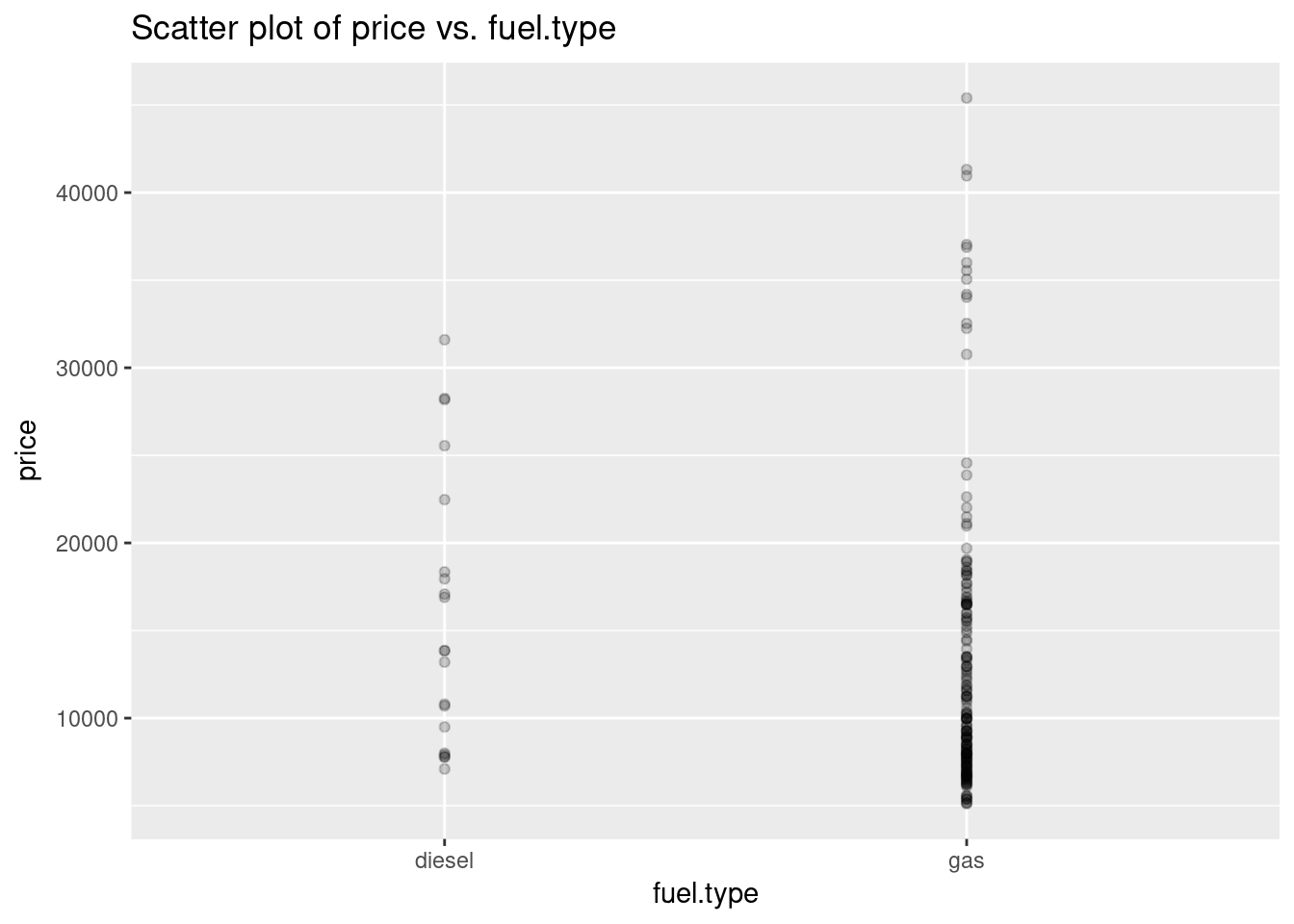
plot_scatter_t <- function(df, cols, col_y = 'price', alpha = 1.0){
    options(repr.plot.width=4, repr.plot.height=3.5) # Set the initial plot area dimensions
    for(col in cols){
        p <- ggplot(df, aes_string(col, col_y)) +
                   geom_point(alpha = alpha) +
                   ggtitle(paste('Scatter plot of', col_y, 'vs.', col))
        print(p)
    }
}

plot_scatter_t(auto_prices, plotcols, alpha = 0.2)
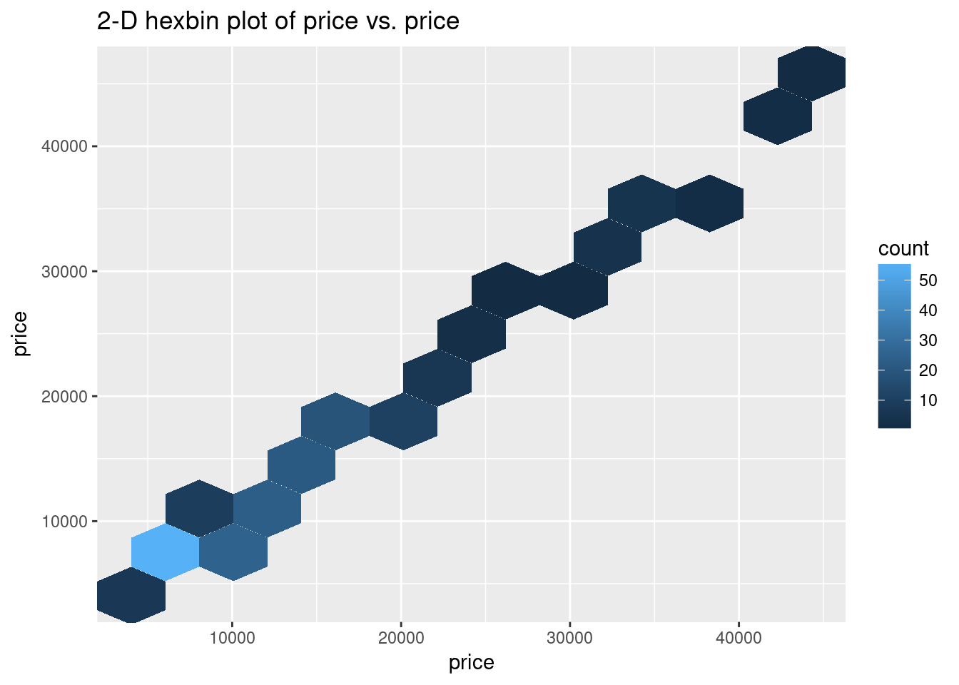
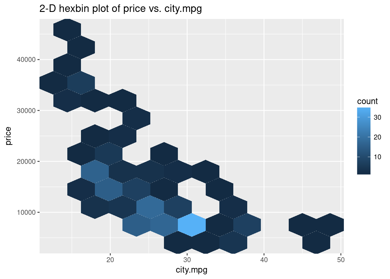
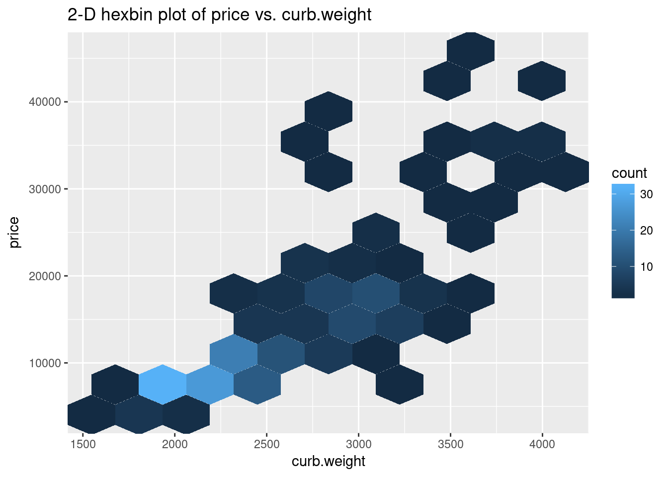
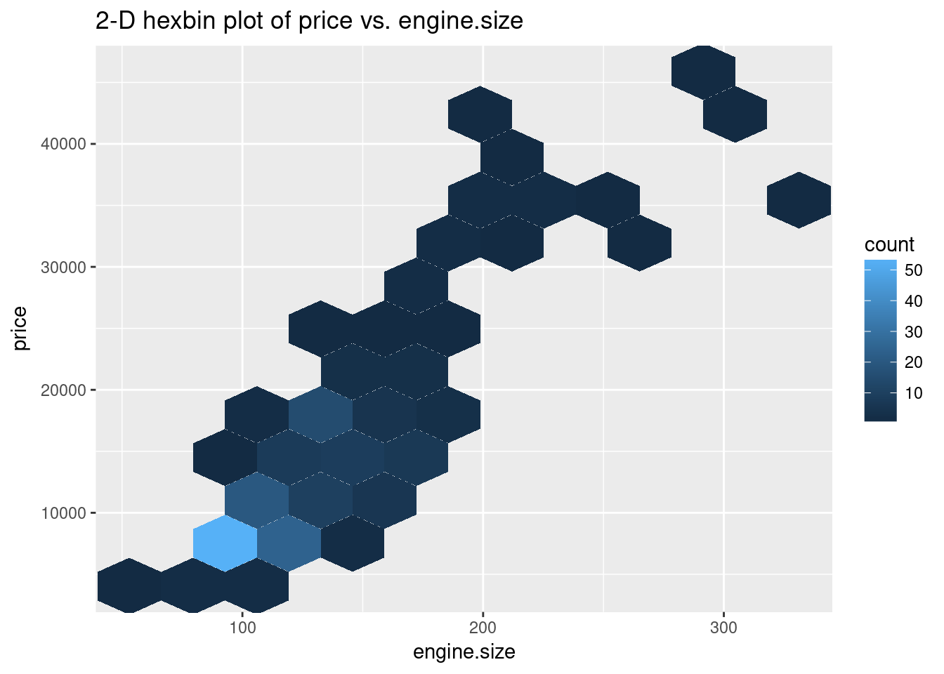
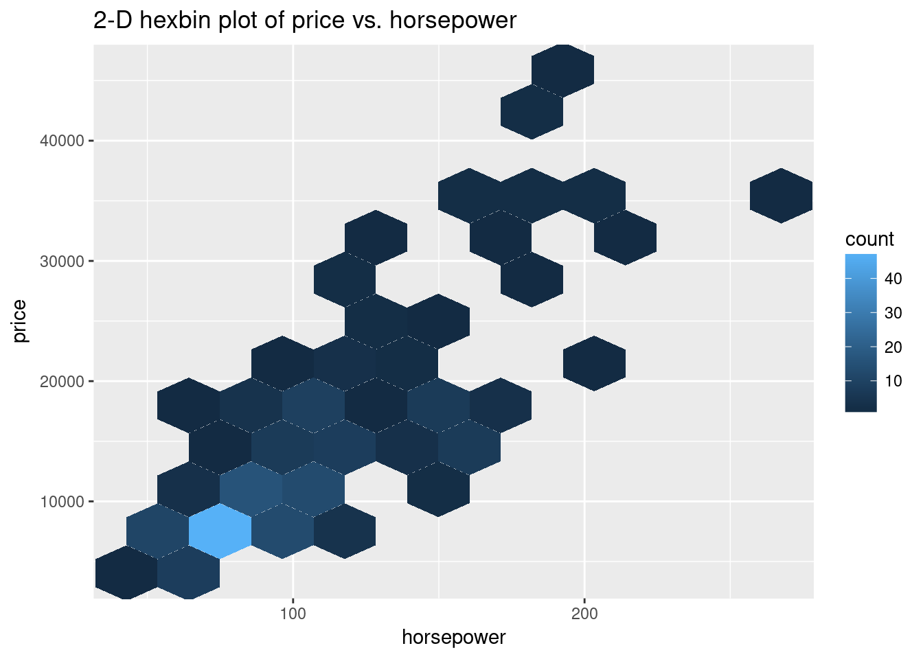
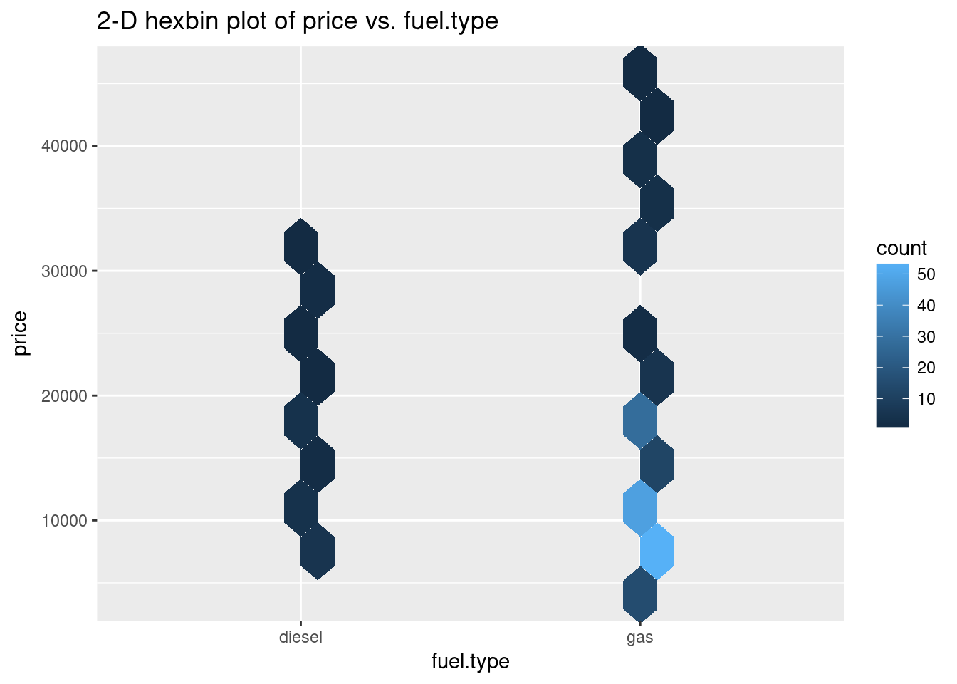
plot_hex <- function(df, cols, col_y = 'price', bins = 30){
    options(repr.plot.width=4, repr.plot.height=3.5) # Set the initial plot area dimensions
    for(col in cols){
        p <- ggplot(df, aes_string(col, col_y)) +
                   geom_hex(show.legend = TRUE, bins = bins) +
                   ggtitle(paste('2-D hexbin plot of', col_y, 'vs.', col))
        print(p)
    }
}

plot_hex(auto_prices, plotcols, bins = 10)
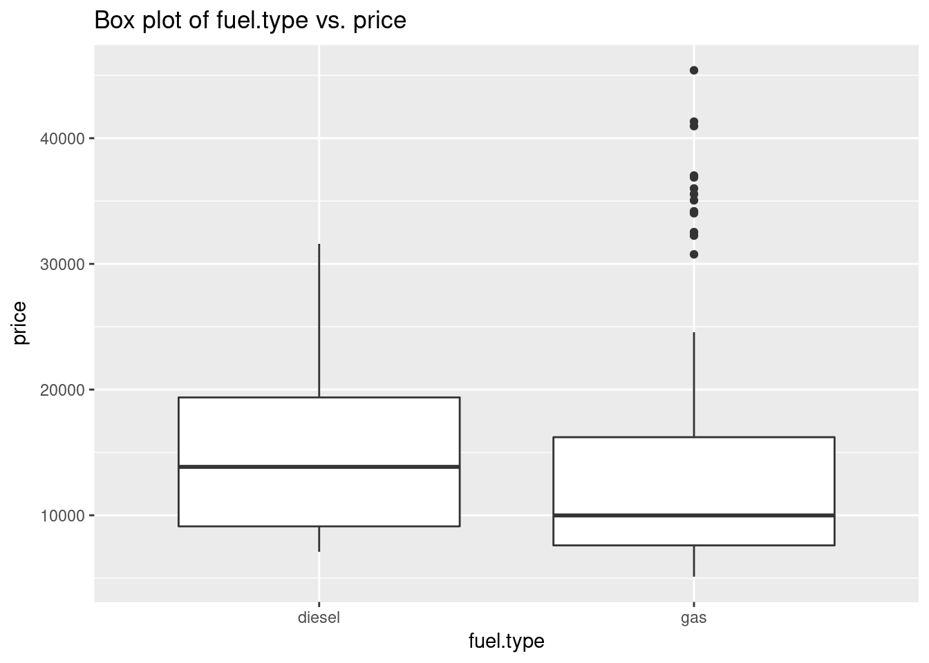
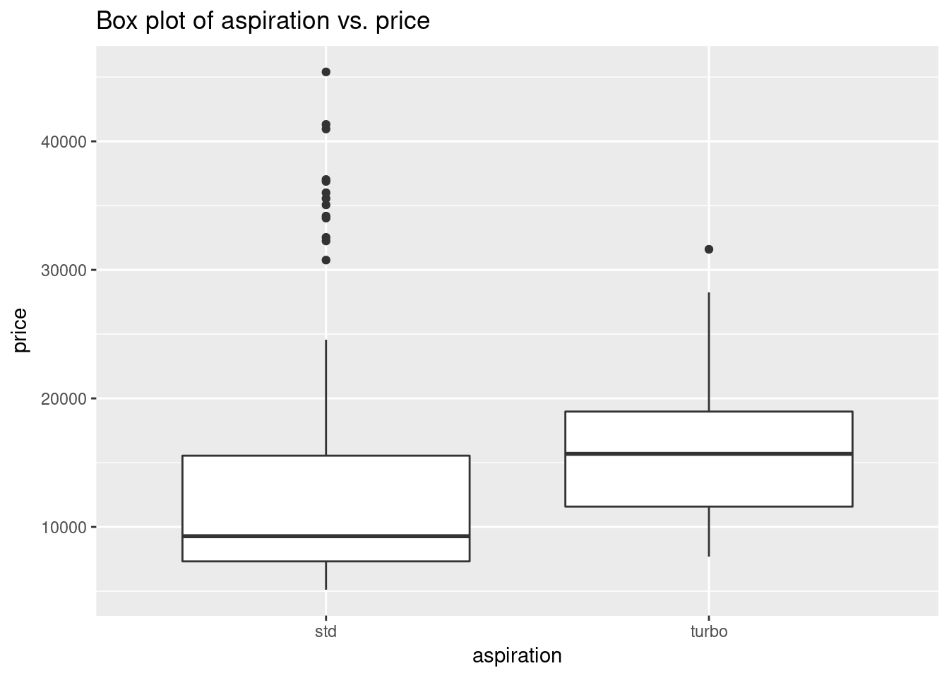
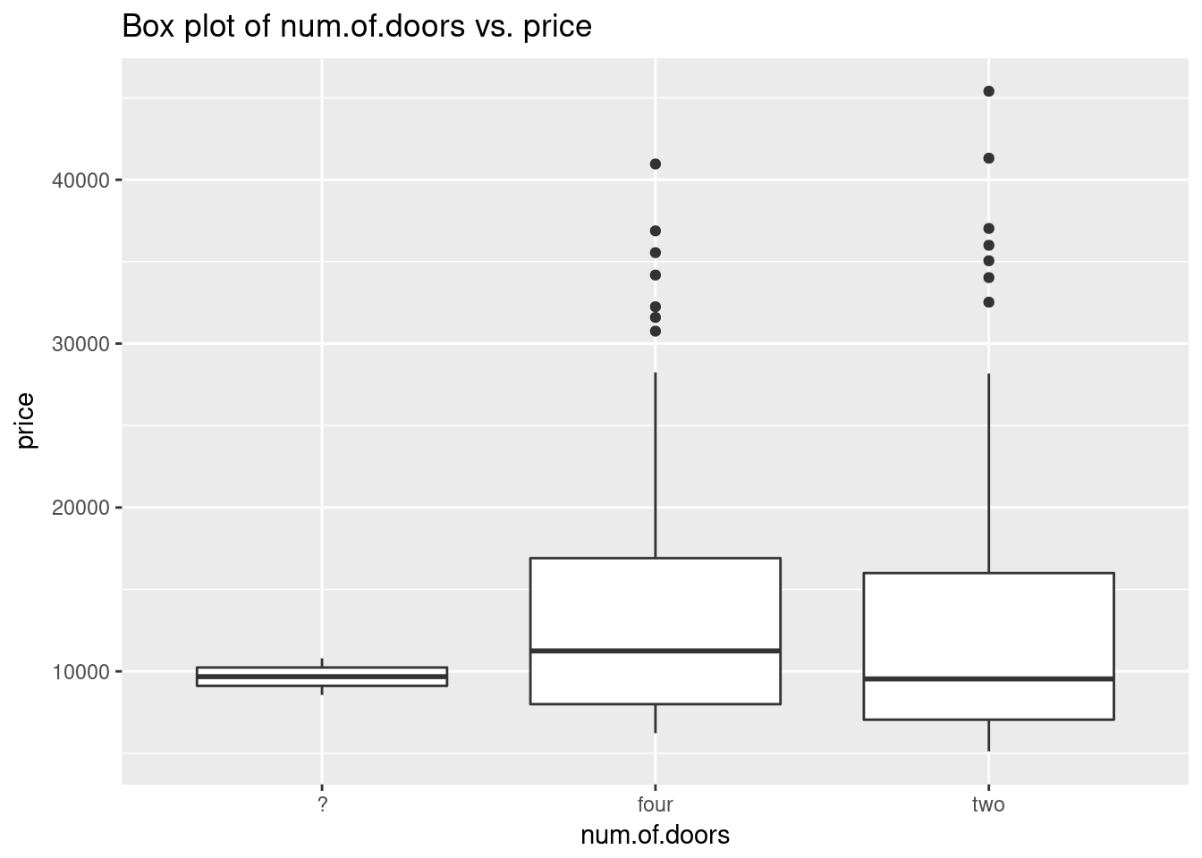
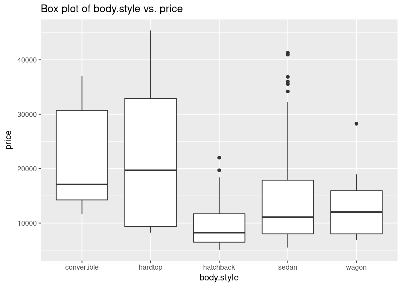
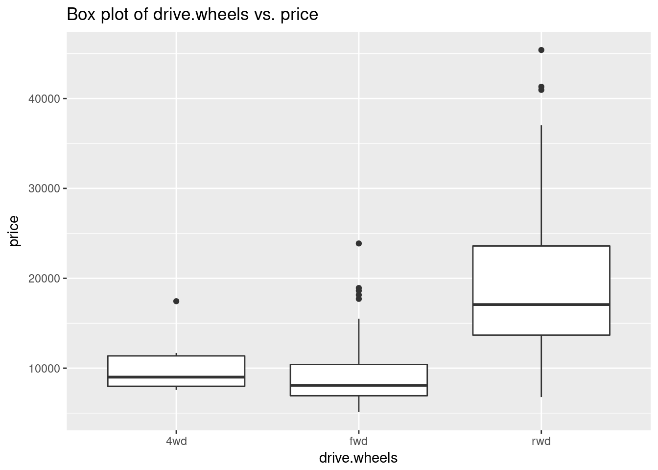
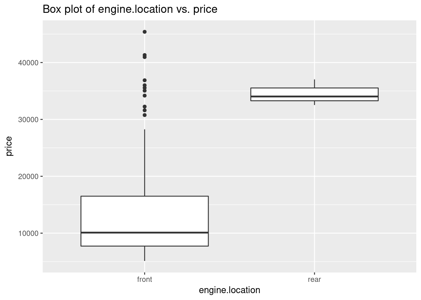
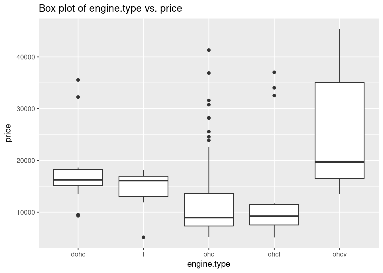
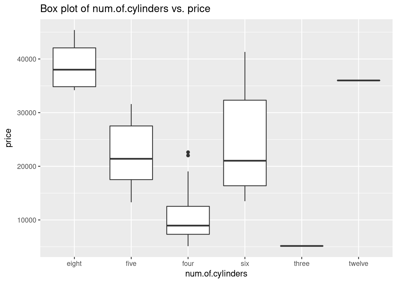
plot_box <- function(df, cols, col_y = 'price'){
    options(repr.plot.width=4, repr.plot.height=3.5) # Set the initial plot area dimensions
    for(col in cols){
        p <- ggplot(df, aes_string(col, col_y)) +
                   geom_boxplot() +
                   ggtitle(paste('Box plot of', col, 'vs.', col_y))
        print(p)
    }
}

plot_box(auto_prices, cat_cols)
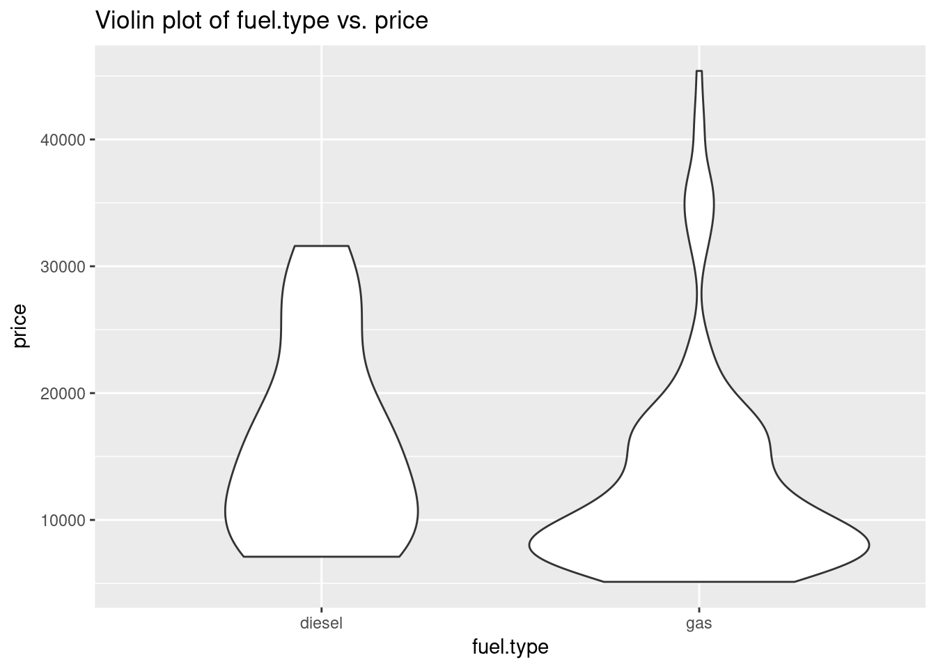
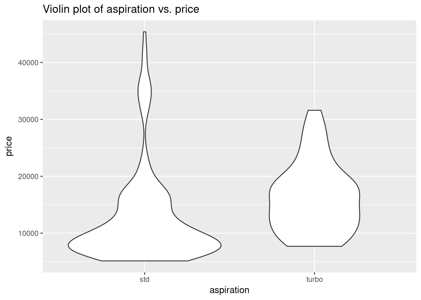
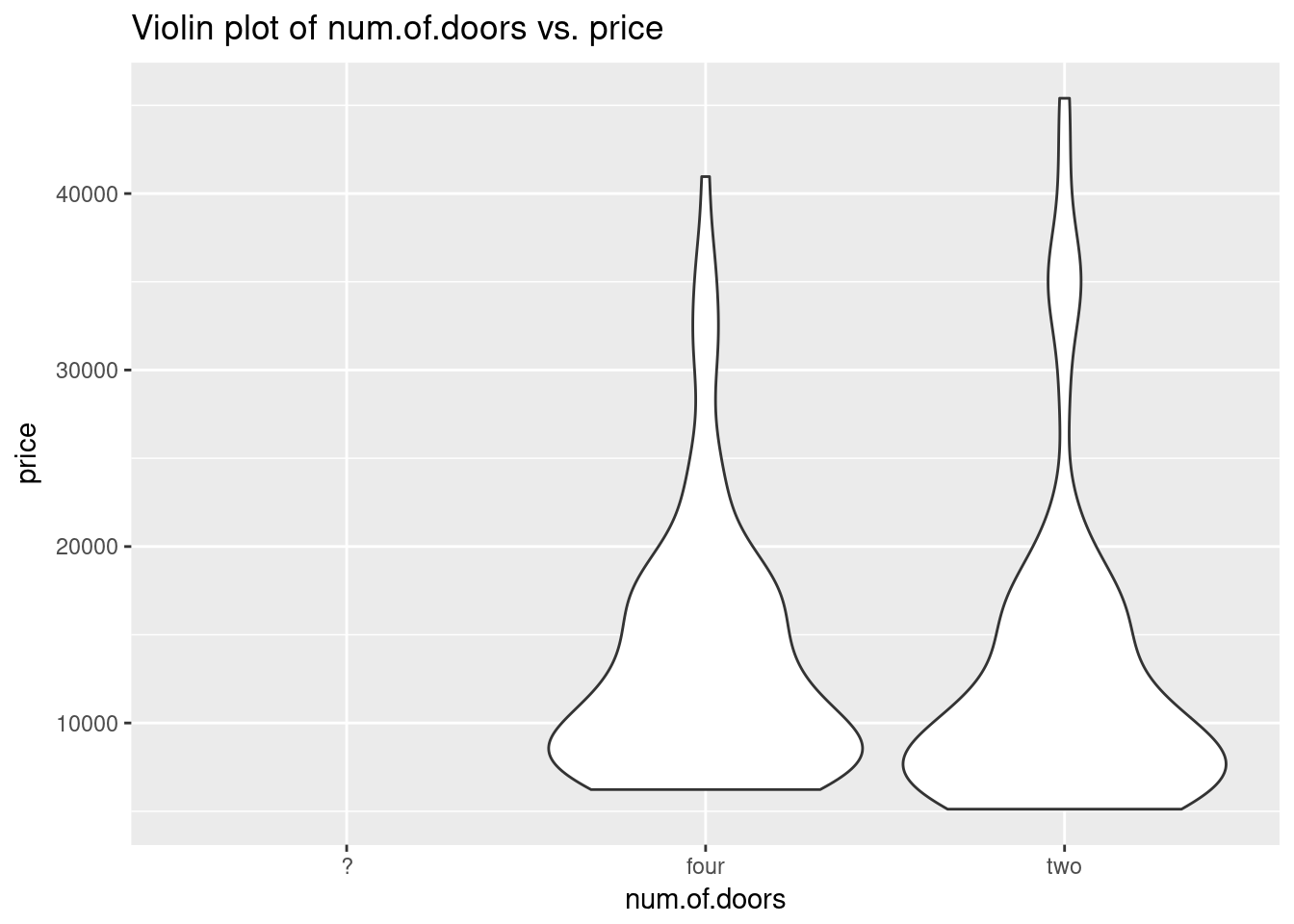
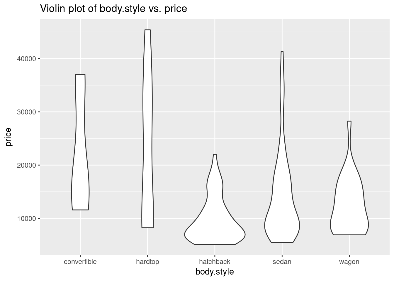
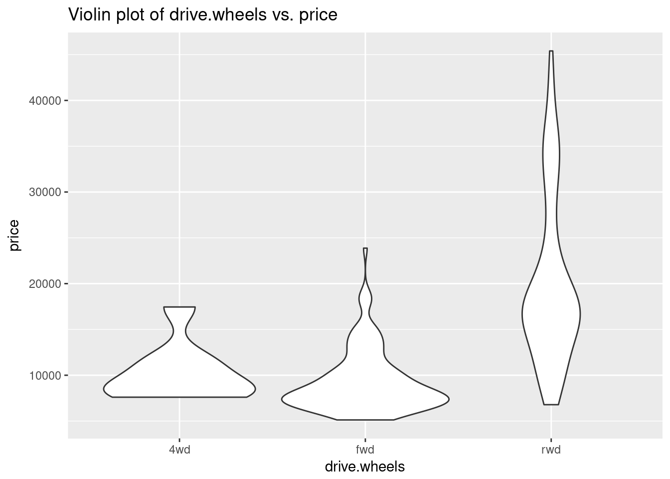
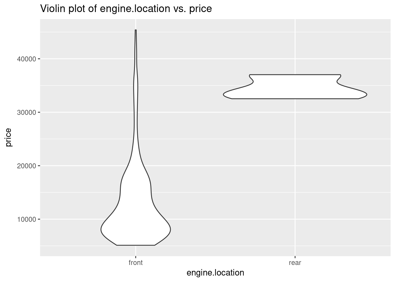
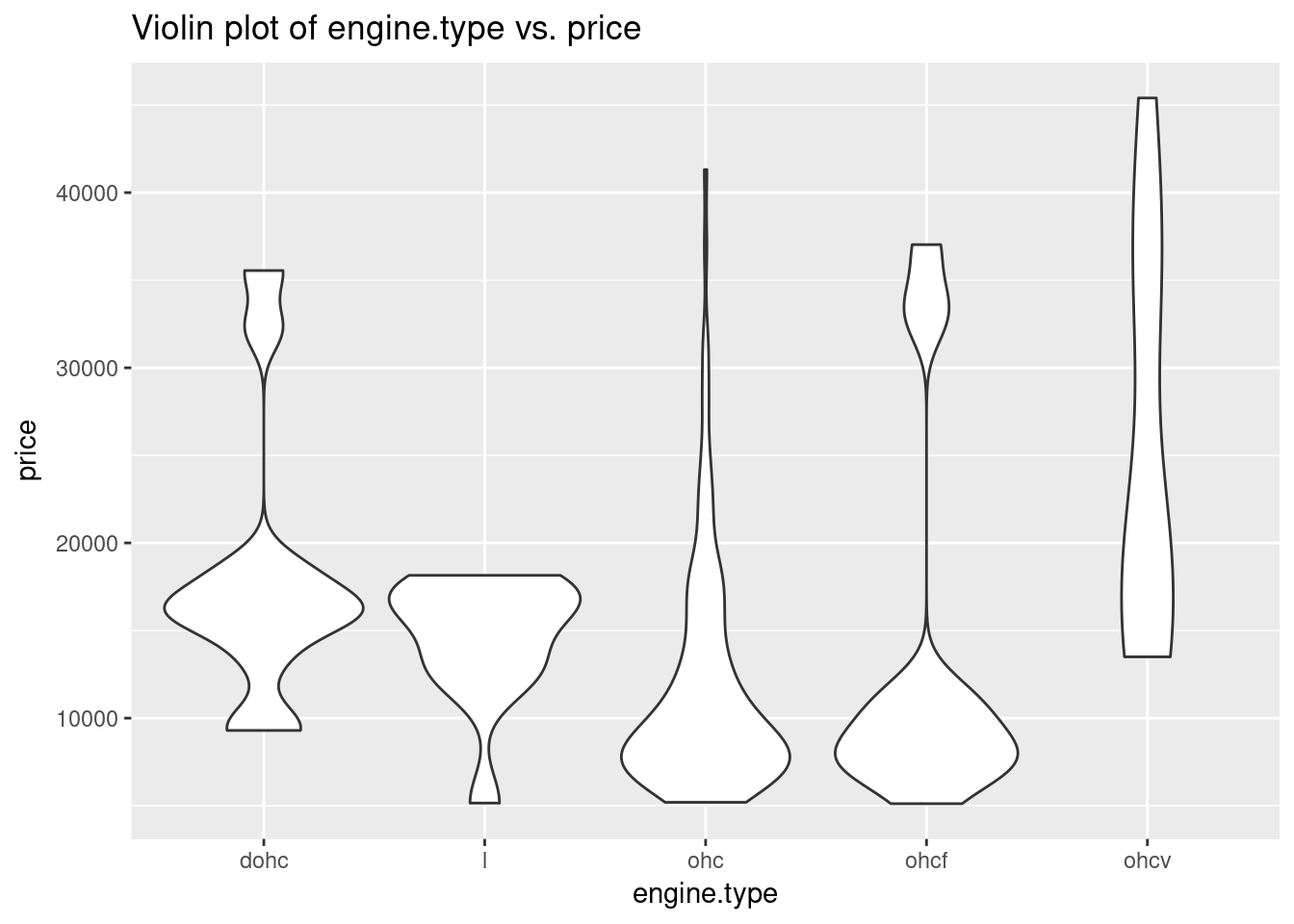
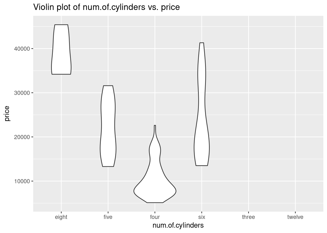
plot_violin <- function(df, cols, col_y = 'price', bins = 30){
    options(repr.plot.width=4, repr.plot.height=3.5) # Set the initial plot area dimensions
    for(col in cols){
        p <- ggplot(df, aes_string(col, col_y)) +
                   geom_violin() +
                   ggtitle(paste('Violin plot of', col, 'vs.', col_y))
        print(p)
    }
}

plot_violin(auto_prices, cat_cols)
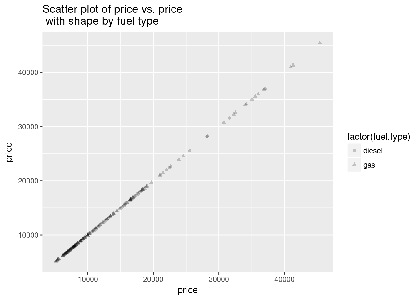
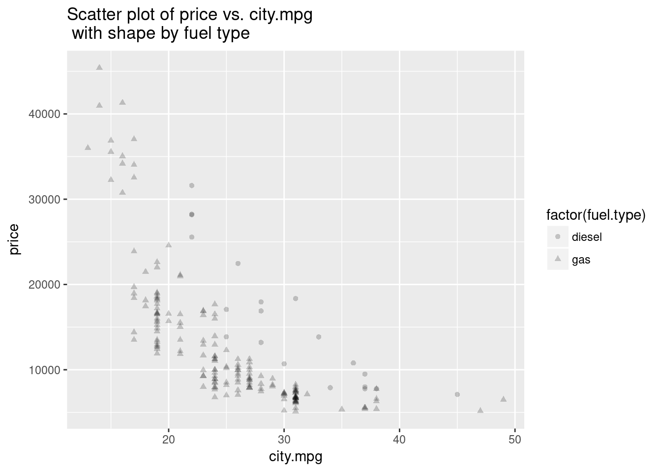
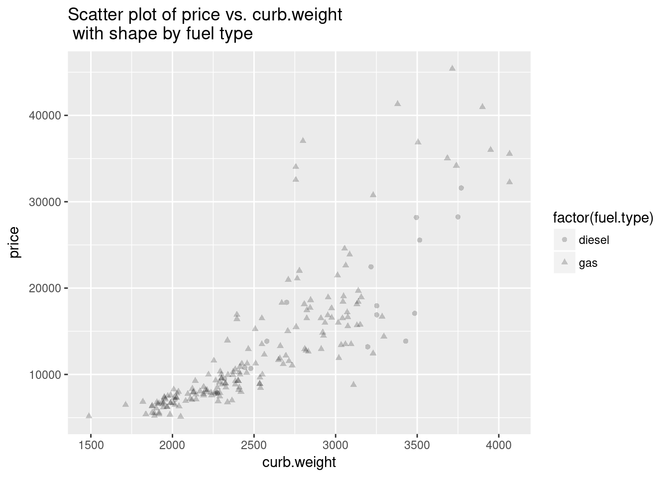
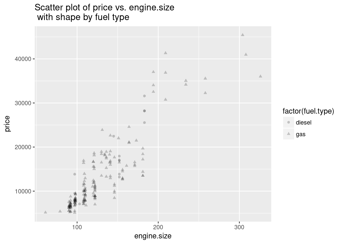
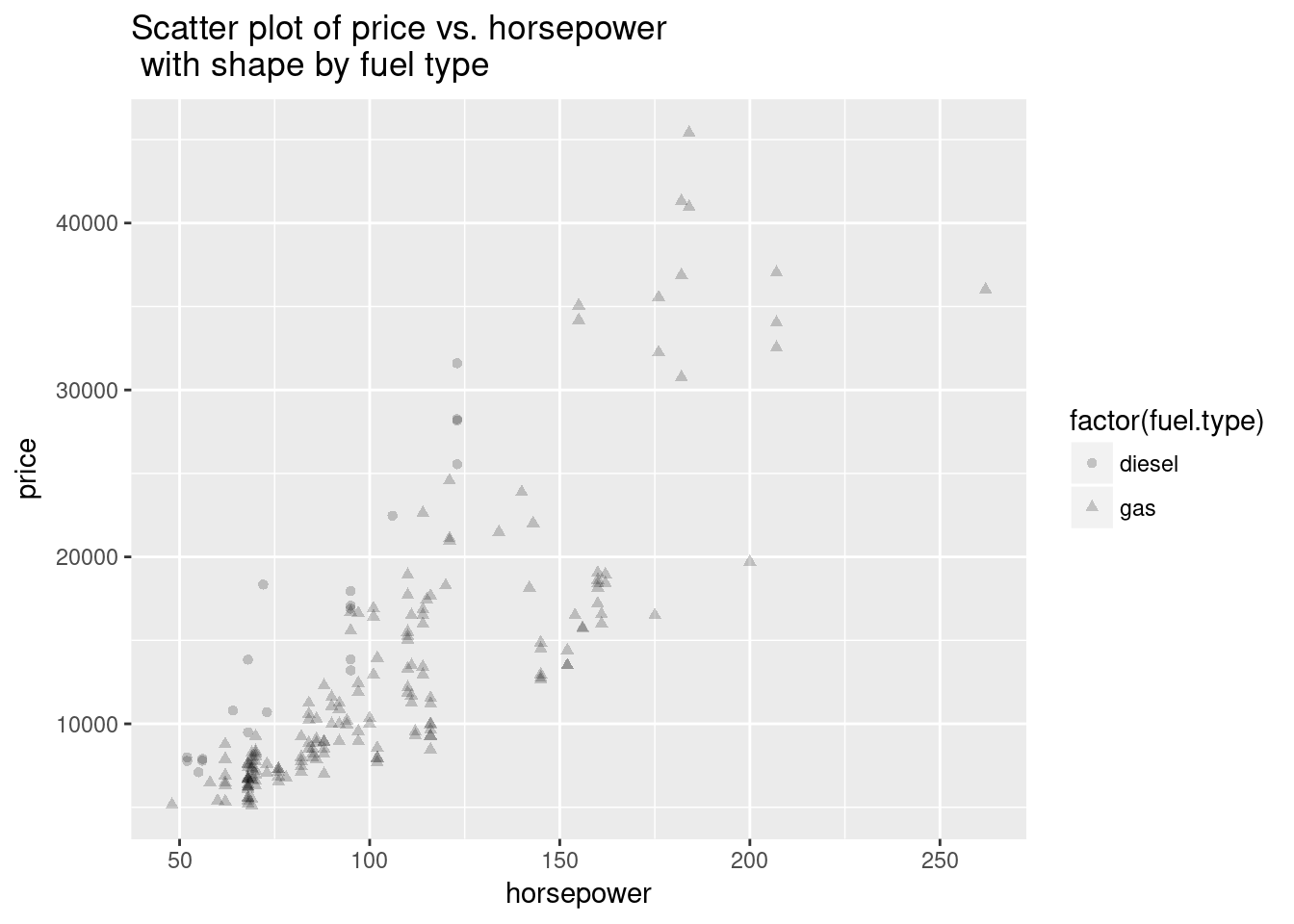
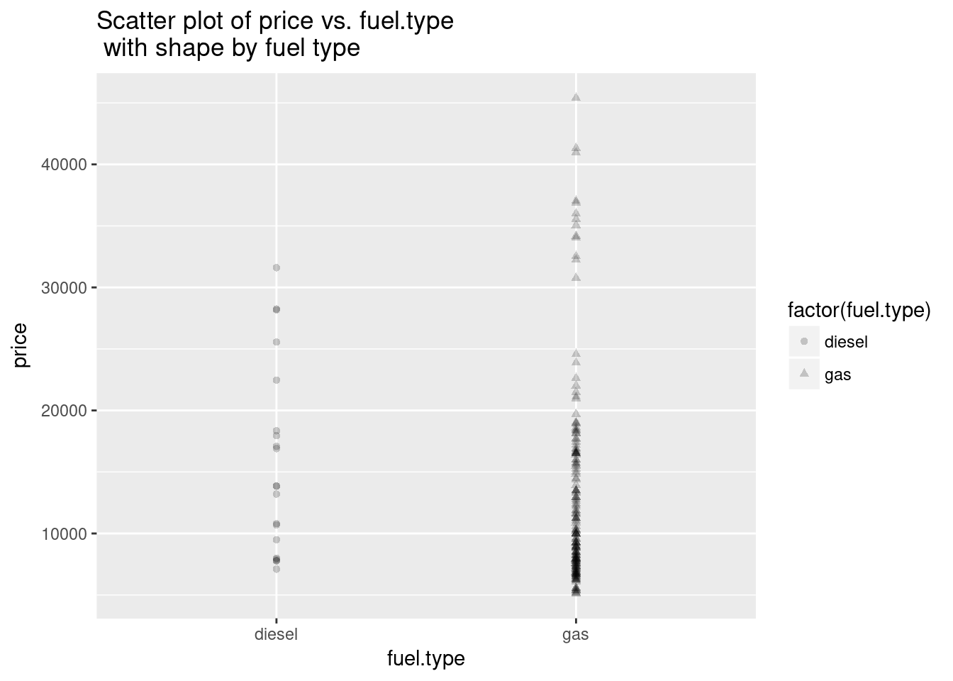
plot_scatter_sp <- function(df, cols, col_y = 'price', alpha = 1.0){
    options(repr.plot.width=5, repr.plot.height=3.5) # Set the initial plot area dimensions
    for(col in cols){
        p <- ggplot(df, aes_string(col, col_y)) +
                   geom_point(aes(shape = factor(fuel.type)), alpha = alpha) +
                   ggtitle(paste('Scatter plot of', col_y, 'vs.', col, '\n with shape by fuel type'))
        print(p)
    }
}

plot_scatter_sp(auto_prices, plotcols, alpha = 0.2)
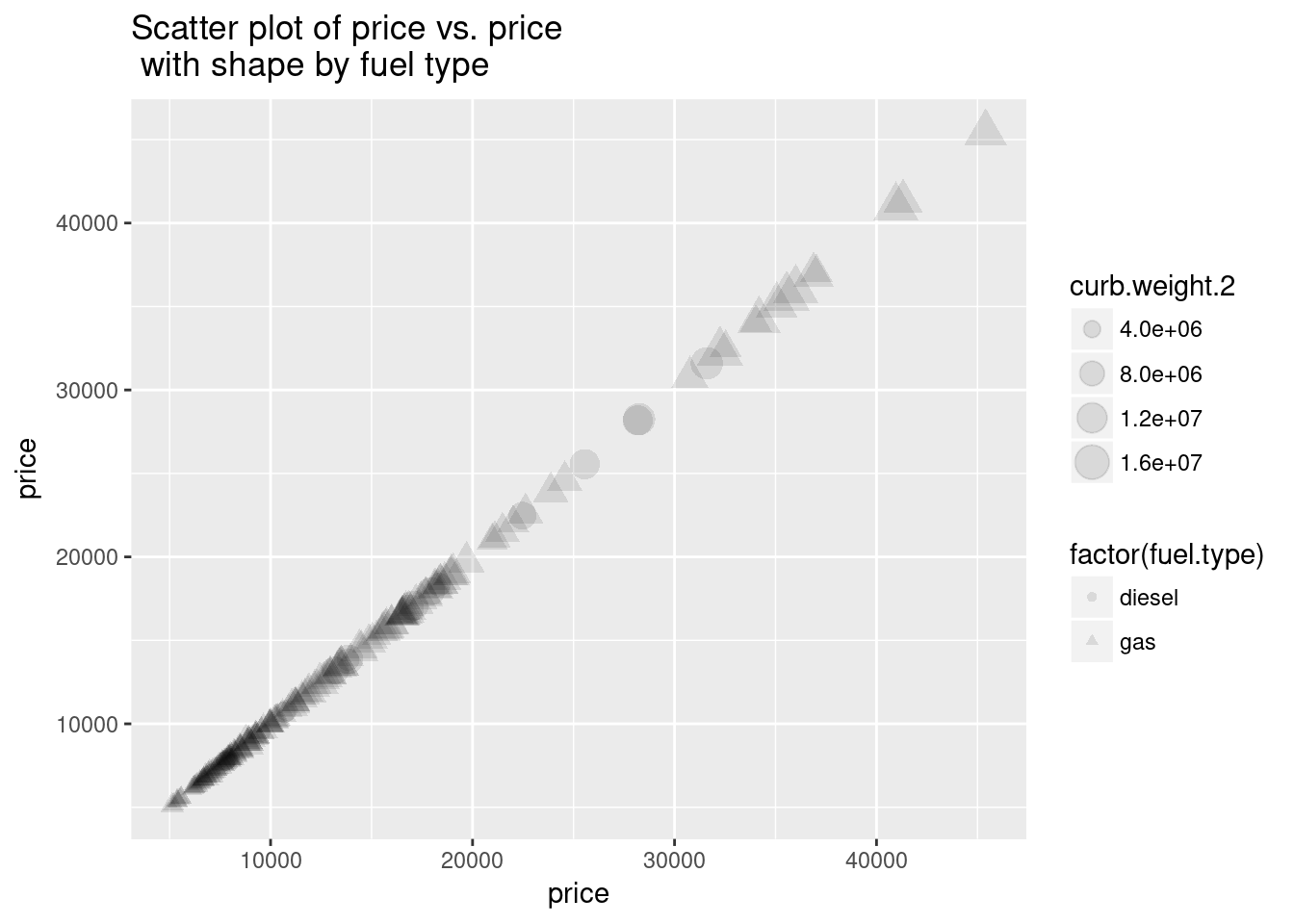
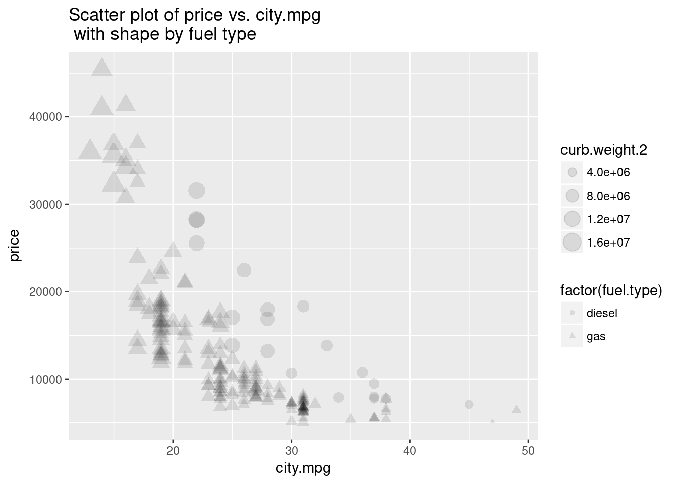
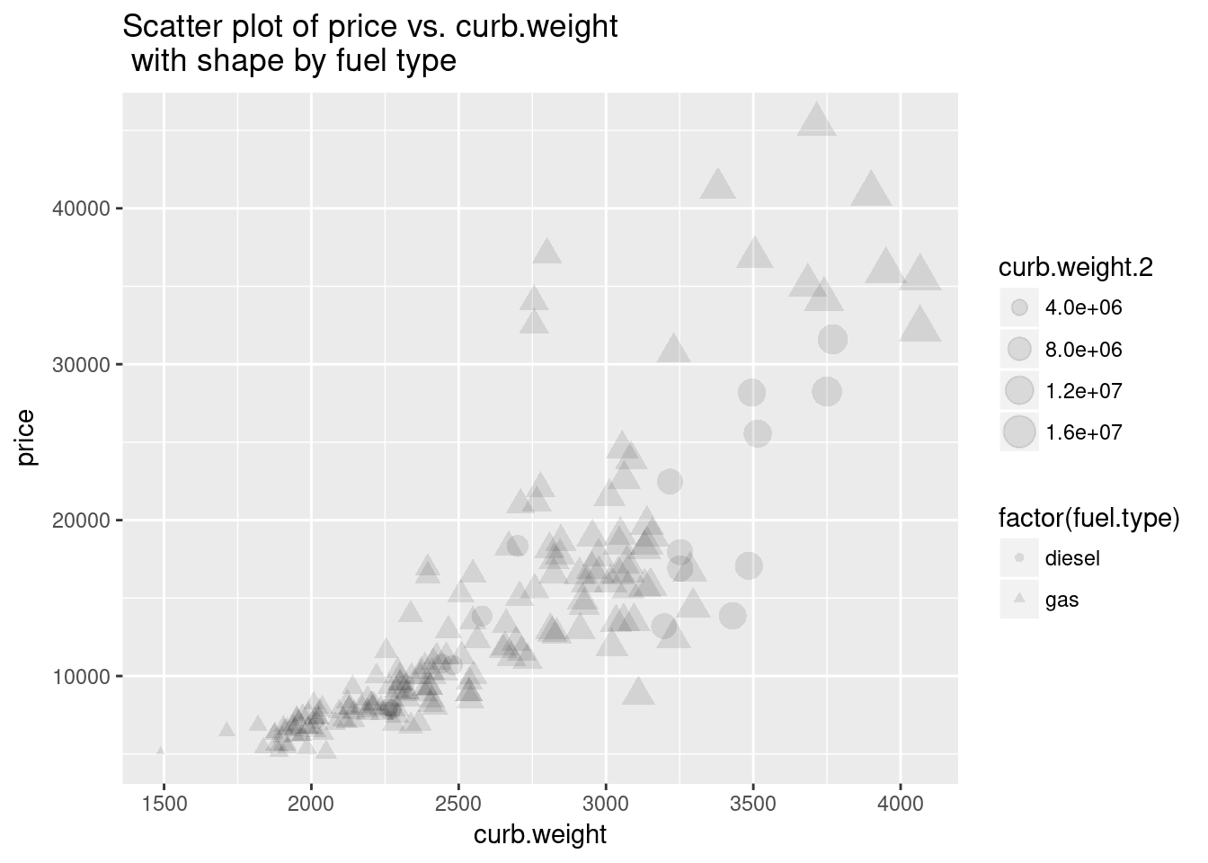
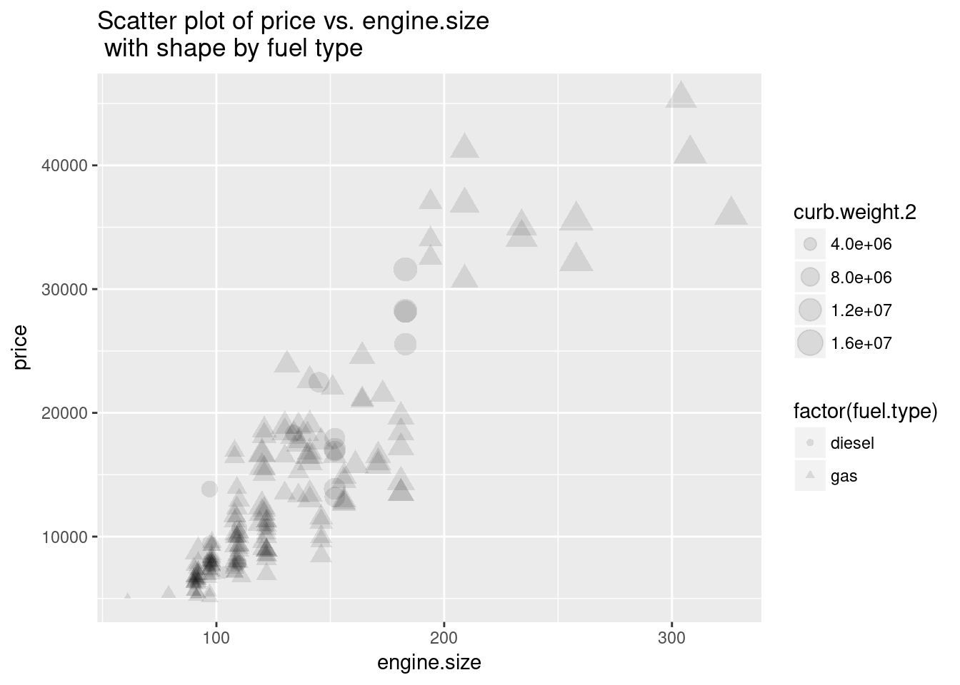
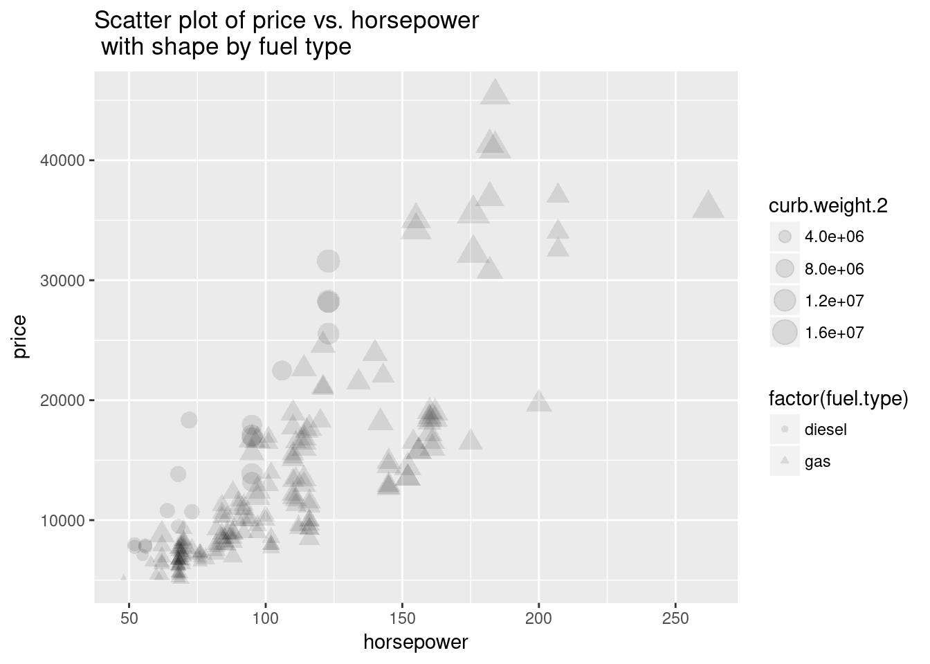
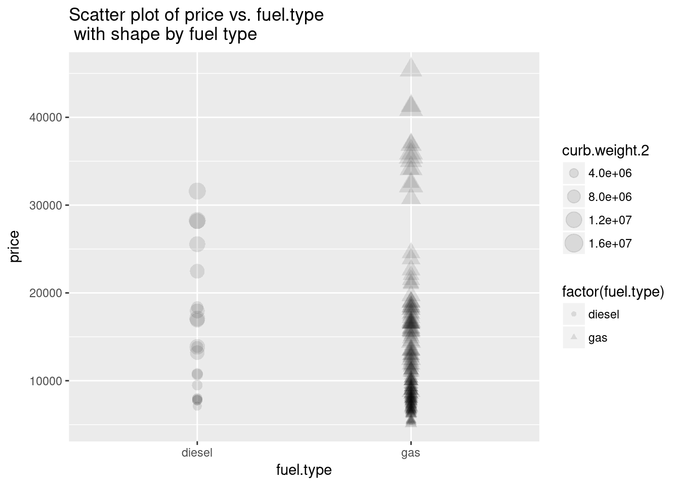
plot_scatter_sp_sz = function(df, cols, col_y = 'price', alpha = 1.0){
    options(repr.plot.width=5, repr.plot.height=3.5) # Set the initial plot area dimensions
    df$curb.weight.2 = df$curb.weight**2
    for(col in cols){
        p = ggplot(df, aes_string(col, col_y)) +
                   geom_point(aes(shape = factor(fuel.type), size = curb.weight.2), alpha = alpha) +
                   ggtitle(paste('Scatter plot of', col_y, 'vs.', col, '\n with shape by fuel type'))
        print(p)
    }
}

plot_scatter_sp_sz(auto_prices, plotcols, alpha = 0.1)
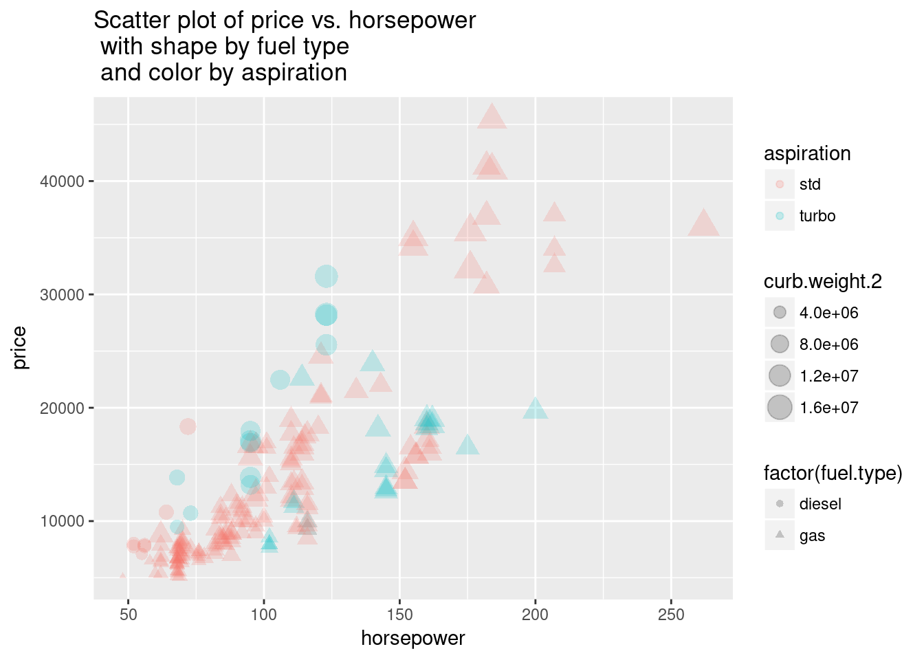
plot_scatter_sp_sz_cl = function(df, cols, col_y = 'price', alpha = 1.0){
    options(repr.plot.width=5, repr.plot.height=3.5) # Set the initial plot area dimensions
    df$curb.weight.2 = df$curb.weight**2
    for(col in cols){
        p = ggplot(df, aes_string(col, col_y)) +
                   geom_point(aes(shape = factor(fuel.type), size = curb.weight.2, color = aspiration),
                              alpha = alpha) +
                   ggtitle(paste('Scatter plot of', col_y, 'vs.', col,
                                 '\n with shape by fuel type',
                                 '\n and color by aspiration'))
        print(p)
    }
}

plot_scatter_sp_sz_cl(auto_prices, plotcols, alpha = 0.2)


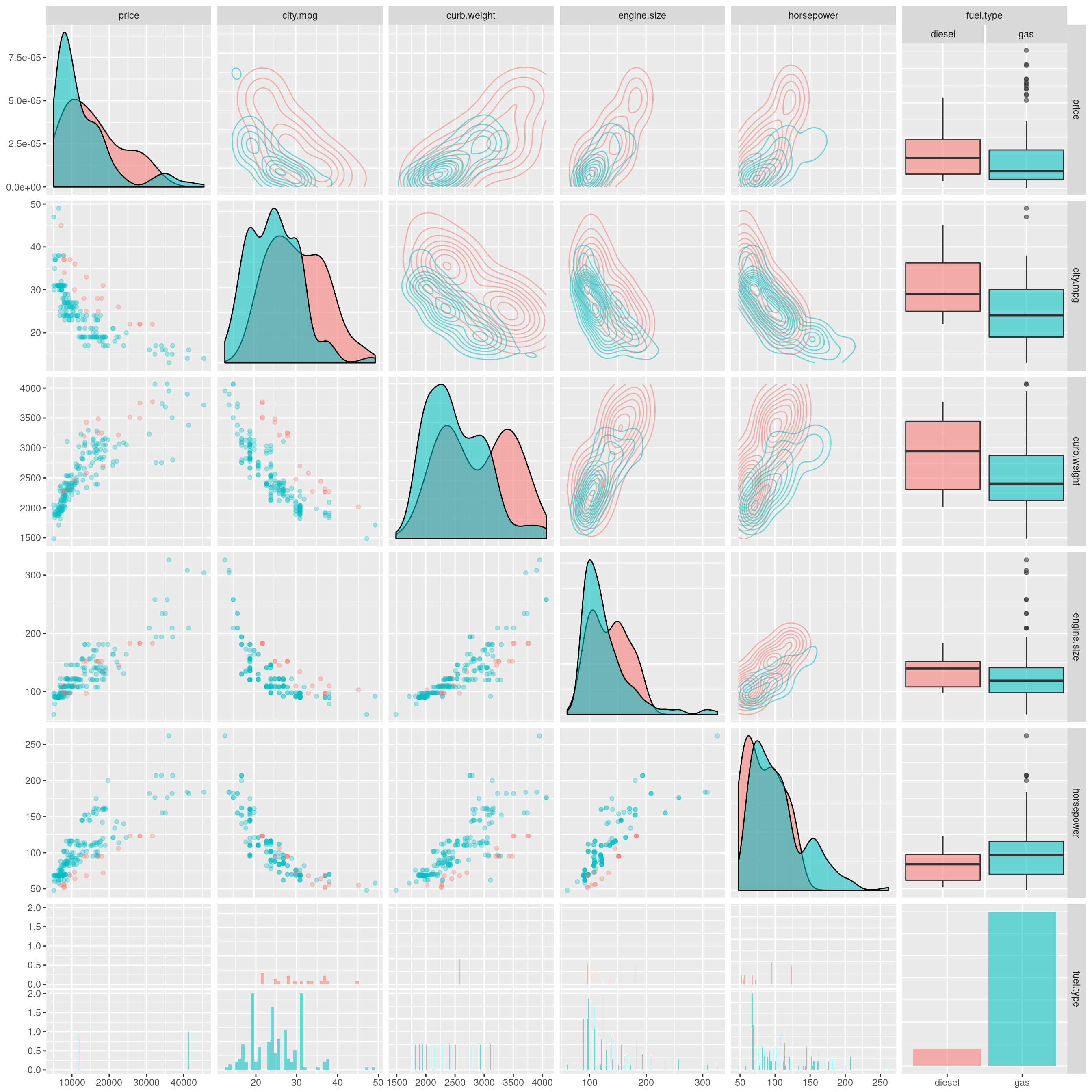
options(repr.plot.width=6, repr.plot.height=6) # Set the initial plot area dimensions
plot_ggp <- ggpairs(auto_prices,
      columns = plotcols,
      aes(color = fuel.type, alpha = 0.1),
      lower = list(continuous = wrap("points", alpha = 0.3), combo = wrap("facethist", binwidth=0.8)),
      upper = list(continuous = ggally_density, combo = wrap("box")),
      progress = FALSE)